Chapter 17 Exercise: Survival estimation

17.1 Introduction to mark-recapture modelling

Recapture or resightings (reencounters) of marked individuals inform about apparent survival, i.e. the probability that an individual survives and stays in the study area. Apparent survival differs from true survival because when the animals is seen last, it is still alive, i.e. the death is not observed. Thus, if an animal is no longer recaptured or resighted, we do not know whether it moved out of the study area or whether it died. Mark-recapture modelling techniques are designed to separately estimate recapture/resighting probability and apparent survival. To do so, they separate the observation process (recapturing or resighting an animal) from the biological process (staying in the study area and surviving). The basis for the development of an immense diversity of mark-recapture models has been set by the Cormack-Jolly-Seber model (Cormack 1964; Jolly 1965; Seber 1965). The CJS-model is introduced here using data on Snowfinches, a high alpine bird species that we study since 2015.

load("data/annualCRdata.rda") # load datax object

Since 2015, we individually marked 1310 Snowfinches. We systematically observed Snowfinches to read rings using scopes and cameras. We could resight 529 of the marked individuals in later years, many of them in more than one year. We collated the marking and resighting data in a capture history matrix \(y\). Each row of \(y\) contains the capture history of one individual and each column corresponds to a year from 2015 to 2023. A \(1\) indicates that the individual was resighted or recaptured during that year and a \(0\) indicates that the individual has not been seen. Thus, a \(1\) means the individual is alive in the study area and it has been detected by the researchers. A \(0\) could mean that the individual died, that it emigrated from the study area or that it is still alive in the study area but has not been detected by the researchers.

index <- order(datax$first)
ch <- datax$y[index,]
plot(c(1,datax$nocc), c(1, datax$nind), type="n", axes=FALSE, xlab="Yeaer", ylab="Individual")
axis(1, at=1:datax$nocc)
axis(2, at=1:datax$nind, las=1, cex.lab=0.5)
for(i in 1:datax$nind){
  points(c(1:datax$nocc)[ch[i,]==1], rep(i,sum(ch[i,])), cex=.6) 
  lines(c(1:datax$nocc)[ch[i,]==1], rep(i,sum(ch[i,])))
}

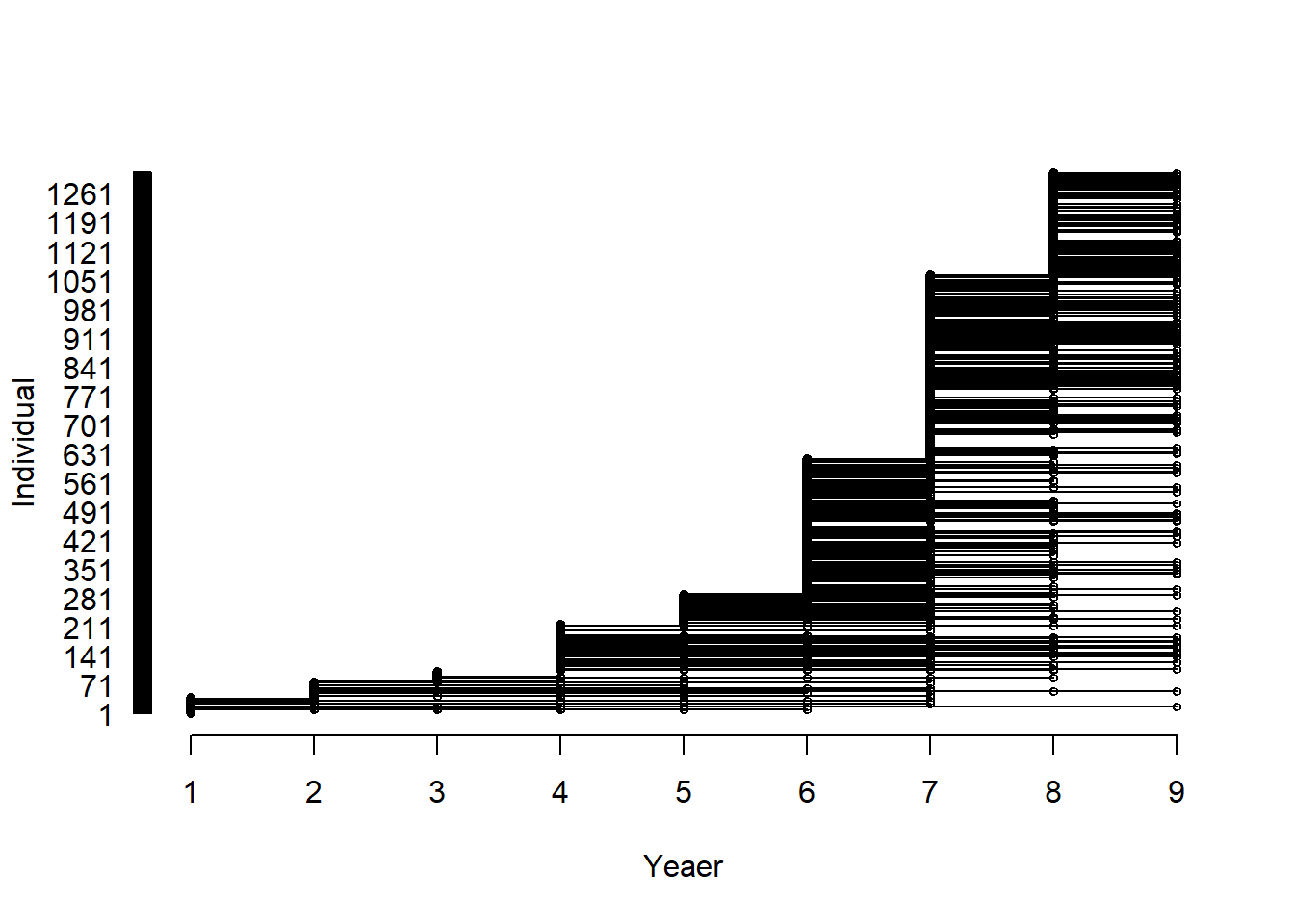
Figure 17.1: Visualisation of the capture-recapture/resighting data. Each horizontal line connect capture or resightings of the same individual, a circle indicate that the individual is captured or resighted at least once during that year.

Model description:

The observations \(y_{it}\), an indicator of whether individual \(i\) was recaptured or resighted during year \(t\) is modeled conditional on the latent true state of the individual birds \(z_{it}\) (0 = dead or permanently emigrated, 1 = alive and at the study site) as a Bernoulli variable. The probability \(P(y_{it} = 1)\) is the product of the probability that an alive individual is recaptured or resighted, \(p_{it}\), and the state of the bird \(z_{it}\) (alive = 1, dead = 0). Thus, a dead bird cannot be recaptured or resighted, whereas for a bird alive during year \(t\), the recapture/resighting probability equals \(p_{it}\): \[y_{it} \sim Bernoulli(z_{it}p_{it})\] The latent state variable \(z_{it}\) is a Markovian variable with the state at year \(t\) being dependent on the state at year \(t-1\) and the apparent survival probability \(\phi_{it}\): \[z_{it} \sim Bernoulli(z_{it-1}\phi_{it})\]

We use the notation \(\phi\) to indicate that this parameter can be interpreted as apparent survival rather than true survival of which the standard notation would be \(S\) (D. L. Thomson et al. 2009). We model \(\phi\) dependent on age (1=first year, 2=older) and year.

\[\phi_{it} = \alpha_{age-class[it], t} \]

Annual recapture/resighting probability is modeled for each year independently: \[p_{it} = \beta_{t}\] We use uniform prior distributions for all parameters with a parameter space limited to values between 0 and 1 (probabilities), \(\alpha_{age-class,t} \sim uniform(0,1)\) and \(\beta_t \sim uniform(0,1)\).

We use Markov chain Monte Carlo simulations as implemented in jags (Plummer 2003) to fit the model to the data. For doing so, we first need to specify the model using Jags language. We do that in a separate text-file (jags/cjs.txt).

To fit the model, the Software jags need to be downloaded and installed.

## ## jags model code
## model{
##   ## likelihood
##   for(i in 1:nind){
##     z[i,first[i]]  <- 1
##     for(t in (first[i]+1):nocc) {
##       phiz[i, t-1] <- z[i,t-1]*phi[i, t-1]
##       z[i,t] ~ dbern(phiz[i, t-1])
##       zp[i,t] <- z[i,t]*p[i,t-1]
##       y[i,t] ~ dbern(zp[i,t])
##     }
##   }
## 
##   ## linear predictors
##   for(i in 1:nind){
##     for(t in first[i]:(nocc-1)){
##       phi[i,t] <-  a[age[i,t],t]
##       p[i,t] <-  b[t]
##     }
##   }
## 
##   ## priors
##  for(t in 1:(nocc-1)){
##   b[t] ~ dunif(0, 1)
##   a[1,t] ~ dunif(0, 1)
##   a[2,t] ~ dunif(0, 1)
## 
##  }
## }

After having specified the model, we need to bundle the data into a list. We have prepared that list in the object datax.

str(datax)
## List of 5
##  $ y    : 'table' num [1:1310, 1:9] 0 1 1 1 1 1 1 1 1 1 ...
##  $ first: int [1:1310] 8 1 1 1 1 1 1 1 1 1 ...
##  $ age  : num [1:1310, 1:9] NA 2 2 1 1 1 1 2 1 1 ...
##  $ nind : int 1310
##  $ nocc : int 9

We then need to specify initial values and the parameters that we would like to save.

library(R2jags)

## Lade nötiges Paket: rjags

## Lade nötiges Paket: coda

## Linked to JAGS 4.3.1

## Loaded modules: basemod,bugs

## 
## Attache Paket: 'R2jags'

## Das folgende Objekt ist maskiert 'package:coda':
## 
##     traceplot

initz <- matrix(NA, ncol=datax$nocc, nrow=datax$nind)
for(i in 1:datax$nind) initz[i,(datax$first[i]+1):datax$nocc] <- 1
initfun <- function(){
  list(a=matrix(runif(2*(datax$nocc-1), 0,1), ncol=datax$nocc-1, nrow=2),
       b=runif(datax$nocc-1, 0,1),
       z=initz)
}


parameters <- c("a", "b")
mod <- jags(datax, inits=initfun, parameters.to.save=parameters, 
            model.file="jags/cjs.txt", n.chains=3, n.iter=2000)

## module glm loaded

## Compiling model graph
##    Resolving undeclared variables
##    Allocating nodes
## Graph information:
##    Observed stochastic nodes: 3726
##    Unobserved stochastic nodes: 3750
##    Total graph size: 28048
## 
## Initializing model

mod <- mod$BUGSoutput

Before we look at the results, we check how well the Markov chains converged. The chains look ok except for the parameters of the last year. For the last year, apparent survival cannot be separated from recapture/resighting probability. Thus, we must expect that these chains do not converge well.

# check 
traceplot(mod)

In the Cormack-Jolly-Seber model, for the last occasion, only the product of survival and recapture probability is estimable. Therefore, for these two parameters, it does not look like the Markov chains have converged.

We then look at the results

mod$summary
##                  mean           sd         2.5%          25%          50%
## a[1,1]   3.448467e-01   0.12702064 1.434765e-01 2.523210e-01 3.290997e-01
## a[2,1]   3.694468e-01   0.19145105 8.795942e-02 2.284626e-01 3.377002e-01
## a[1,2]   3.919284e-01   0.14446243 1.574866e-01 2.875741e-01 3.741098e-01
## a[2,2]   5.662439e-01   0.14072879 3.243856e-01 4.634588e-01 5.554819e-01
## a[1,3]   5.322271e-02   0.05452965 1.447030e-03 1.554022e-02 3.706045e-02
## a[2,3]   8.033479e-01   0.13039552 5.056511e-01 7.195101e-01 8.196825e-01
## a[1,4]   1.771219e-01   0.11122393 2.346298e-02 9.281542e-02 1.571861e-01
## a[2,4]   5.195875e-01   0.05397123 4.219096e-01 4.824624e-01 5.166542e-01
## a[1,5]   4.074475e-01   0.14190784 1.551053e-01 3.078900e-01 3.949343e-01
## a[2,5]   7.305560e-01   0.06117338 6.068620e-01 6.906502e-01 7.302820e-01
## a[1,6]   1.346118e-01   0.06361259 3.959281e-02 8.741728e-02 1.266628e-01
## a[2,6]   5.933890e-01   0.03089401 5.361230e-01 5.717235e-01 5.927342e-01
## a[1,7]   9.702990e-02   0.08861313 2.971977e-03 3.173224e-02 7.192013e-02
## a[2,7]   4.551854e-01   0.02682666 4.050685e-01 4.370716e-01 4.547238e-01
## a[1,8]   5.054132e-02   0.05025745 1.420554e-03 1.492257e-02 3.461383e-02
## a[2,8]   7.528513e-01   0.14250024 5.141806e-01 6.271319e-01 7.495710e-01
## b[1]     4.004956e-01   0.15385056 1.491244e-01 2.793051e-01 3.856520e-01
## b[2]     4.062317e-01   0.10948405 2.073028e-01 3.267118e-01 4.030018e-01
## b[3]     5.691697e-01   0.11482802 3.530126e-01 4.874773e-01 5.689789e-01
## b[4]     7.176762e-01   0.06716995 5.787164e-01 6.722516e-01 7.193512e-01
## b[5]     6.374781e-01   0.05858633 5.258354e-01 5.970776e-01 6.391182e-01
## b[6]     8.824514e-01   0.03314925 8.106117e-01 8.614558e-01 8.849537e-01
## b[7]     7.267730e-01   0.03764278 6.484260e-01 7.018844e-01 7.272154e-01
## b[8]     5.949782e-01   0.12299926 4.160904e-01 4.914490e-01 5.735195e-01
## deviance 1.335830e+03 149.67816284 1.026231e+03 1.226483e+03 1.352377e+03
##                   75%        97.5%     Rhat n.eff
## a[1,1]   4.183946e-01    0.6395755 1.002567   970
## a[2,1]   4.780424e-01    0.8399393 1.002345  1100
## a[1,2]   4.785407e-01    0.7200668 1.002704   910
## a[2,2]   6.586373e-01    0.8758056 1.003254   730
## a[1,3]   7.309738e-02    0.1881959 1.002890   840
## a[2,3]   9.074788e-01    0.9892535 1.008109   410
## a[1,4]   2.384160e-01    0.4446621 1.002061  1300
## a[2,4]   5.555184e-01    0.6353294 1.000550  3000
## a[1,5]   5.018983e-01    0.7119856 1.001344  2400
## a[2,5]   7.697637e-01    0.8523710 1.003867   600
## a[1,6]   1.709864e-01    0.2896743 1.001912  1400
## a[2,6]   6.142028e-01    0.6542693 1.000705  3000
## a[1,7]   1.379511e-01    0.3327742 1.002550   980
## a[2,7]   4.729660e-01    0.5084351 1.004390   600
## a[1,8]   6.990244e-02    0.1855901 1.002207  1200
## a[2,8]   8.812083e-01    0.9839843 1.065800    43
## b[1]     5.061958e-01    0.7307027 1.003749   620
## b[2]     4.810474e-01    0.6297698 1.004185   540
## b[3]     6.507282e-01    0.7848872 1.003124   840
## b[4]     7.643689e-01    0.8414163 1.002045  1300
## b[5]     6.773678e-01    0.7547749 1.001679  1700
## b[6]     9.064596e-01    0.9388350 1.002337  1100
## b[7]     7.526649e-01    0.7985460 1.004190   540
## b[8]     6.867156e-01    0.8563174 1.061618    51
## deviance 1.452318e+03 1580.0264073 1.060715    57

plot(c(2015,2023), c(0,1), type="n", las=1, xlab=NA, ylab="Apparent survival")

phi <- apply(mod$sims.list$a, c(2,3), mean)
phi.lwr <- apply(mod$sims.list$a, c(2,3), quantile, probs=0.025)
phi.upr <- apply(mod$sims.list$a, c(2,3), quantile, probs=0.975)
x <- seq(2015.5, 2022.5, by=1)
segments(x, phi.lwr[1,], x,phi.upr[1,])
points(x, phi[1,], pch=21, bg="white")
segments(x+0.1, phi.lwr[2,], x+0.1,phi.upr[2,], lwd=2, col="brown")
points(x+0.1, phi[2,], pch=21, bg="white", col="brown")
legend(2015, 1.1, xpd=NA, lwd=c(1,2), col=c(1,"brown"), legend=c("first year", "adult"), horiz=TRUE)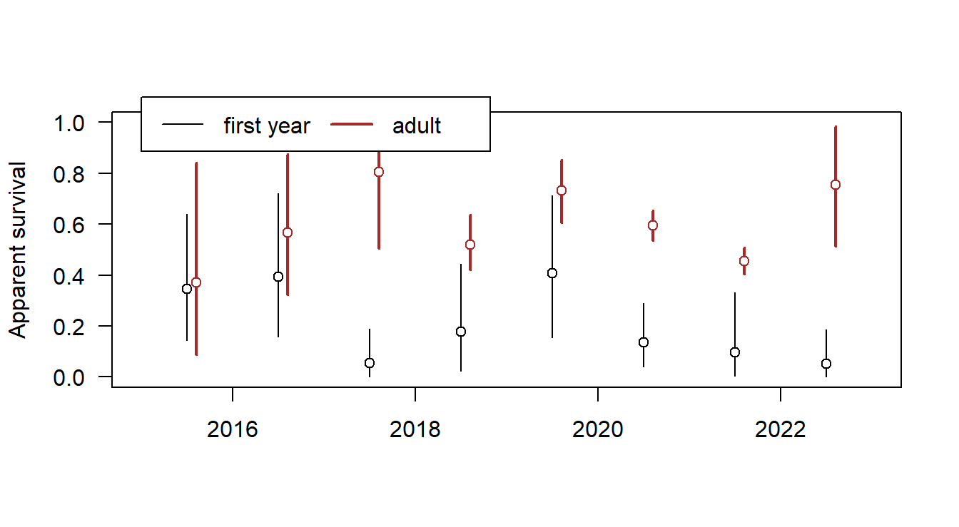

Figure 17.2: Annual apparent survival of juvenile and adult Snowfinches.

plot(c(2016,2023), c(0,1), type="n", las=1, xlab=NA, ylab="Recapture/resighting probability")

p <- apply(mod$sims.list$b, 2, mean)
p.lwr <- apply(mod$sims.list$b, 2, quantile, probs=0.025)
p.upr <- apply(mod$sims.list$b, 2, quantile, probs=0.975)
x <- seq(2016, 2023, by=1)
segments(x, p.lwr, x,p.upr, lwd=2, col="brown")
points(x, p, pch=21, bg="white", col="brown")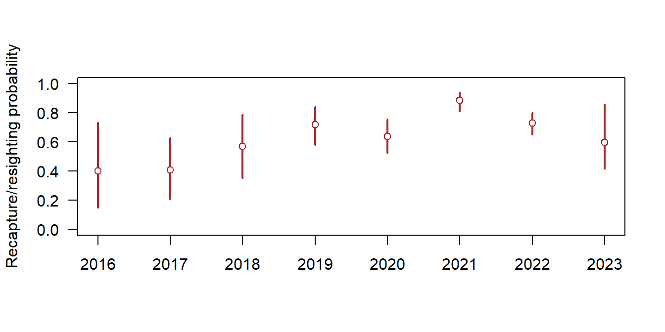

Figure 17.3: Recapture and resighting probability

Kéry and Schaub (2012) wrote a gentle introduction to mark-recapture modelling for biologists. An example using Stan is found here https://tobiasroth.github.io/BDAEcology/cjs_with_mix.html.

References

Cormack, R. M. 1964. “Estimates of Survival from the Sighting of Marked Animals.” Biometrika 51: 429–38.

Jolly, G. 1965. “Explicit Estimates from Capture-Recapture Data with Both Death and Immigration-Stochastic Model.” Biometrika 52: 225–47.

Kéry, Marc, and Michael Schaub. 2012. Bayesian Population Analysis Using WinBUGS. Amsterdam: Elsevier.

Plummer, Martyn. 2003. “JAGS : A Program for Analysis of Bayesian Graphical Models Using Gibbs Sampling JAGS : Just Another Gibbs Sampler.” In Proceedings of the 3rd International Workshop on Distributed Statistical Computing, edited by K. Hornik, F. Leisch, and A. Zeileis, 1–8. Dsc. Vienna.

Seber, G. A. F. 1965. “A Note on the Multiple-Recapture Census.” Biometrika 52: 249–59.

Thomson, D L, M J Conroy, D R Anderson, K P Burnham, E G Cooch, C M Francis, J.-D. Lebreton, et al. 2009. “Standardising Terminology and Notation for the Analysis of Demographic Processes in Marked Populations.” Edited by D L Thomson, E G Cooch, and M J Conroy. Modeling Demographic Processes in Marked Populations, 1099–1106.