Chapter 13 Exercise: Refreshing R and linear models

13.1 Refreshing R

13.1.1 Software installation

Download R and RStudio.

Install the packages rmarkdown, bookdown, knitr, dplyr, tidyr, ggplot2and arm by typing install.packages("rmarkdown") etc. in the R-console. R-packages need to be installed only once, or after a major update of R.

install.packages(c("rmarkdown", "bookdown", "knitr", "dplyr", "tidyr", "ggplot2",  "arm", "bookdown"))

13.1.2 Working with R

Writing and editing code is done in a text editor such as Wordpad or RStudio. RStudio is recommended because it is developed by the R development core team, it understands the R language and it communicates with R.
We write the code in the text file (.r or .rmd) and send it to the R-console in RStudio using ctrl + enter.

13.1.3 Working with rmarkdown

Rmarkdown allows knitting text with R code. The option to knit text with R code allows to write analyses reports without having to copy and paste results from the R console into a Word file. We can optionally show or hide R code and insert results directly in the text. Further, for sharing R code, it is extremely helpful to describe what the R code does in the text sections.

Text is written in plain. Latex notation can be used. Helpful introductions exist online.

R code is written within R chunks. In the header of the R chunks we can specify how the code, results and messages are shown in the output file. By pushing the “Knit” button all R-code is executed and displayed within a html, pdf or word document together with the text. The output format is specified in the header of the rmd-file.

The R-console is the calculator. R can be used as a simple calculator or we can create objects, such as x and apply functions such as mean() to the objects. Functions are followed by round brackets () whithin which we can provide arguments. In the help file of the functions (open by ? followed by the name of the function), we can see what arguments a function needs and what default values the arguments have.

# This is R-code, therefore text is outcommented by the hash-tag sign

36/5  # a mathematical expression
## [1] 7.2

x <- c(4,7,3,6,2,7,4,3,4,6,2,8) # a vector, 
# x becomes an object in the R global environment

mean(x) # apply a function to an object
## [1] 4.666667

# arguments of functions are defined with a specific order
mean(4,7,3,6,2,7,4,3,4,6,2,8) # is not correct!
## [1] 4
# but
mean(c(4,7,3,6,2,7,4,3,4,6,2,8)) # is correct
## [1] 4.666667

# check  ?mean  for arguments, order of arguments and default values

13.2 Linear regression

13.2.1 Theory

You find the theory to this exercise in Chapter 11 in the online book Bayesian Data Analyses Using Linear Models in R and Stan.

13.2.2 Fitting a Linear Regression in R

library(arm)

## Warning: Paket 'Matrix' wurde unter R Version 4.2.3 erstellt

library(dplyr)

## Warning: Paket 'dplyr' wurde unter R Version 4.2.3 erstellt

library(tidyr)
library(ggplot2)

## Warning: Paket 'ggplot2' wurde unter R Version 4.2.3 erstellt

13.2.3 Data

We use weight data of snowfinches Montifringilla nivalis that have been captured and ringed during the winter months and we ask how the average weight changes with the time of the day.

dat <- read.table("data/SFringlistwinter.txt", header=TRUE, sep="\t")
# select winter month
dat <- dat[is.element(dat$month, c(0:3)),]

dat$time.num <- dat$time_hour + dat$time_min/60
plot(dat$time.num, dat$weight, xlab="Hour", ylab="Weight [g]", pch=16, col=rgb(0,0,0,0.5), cex=0.7)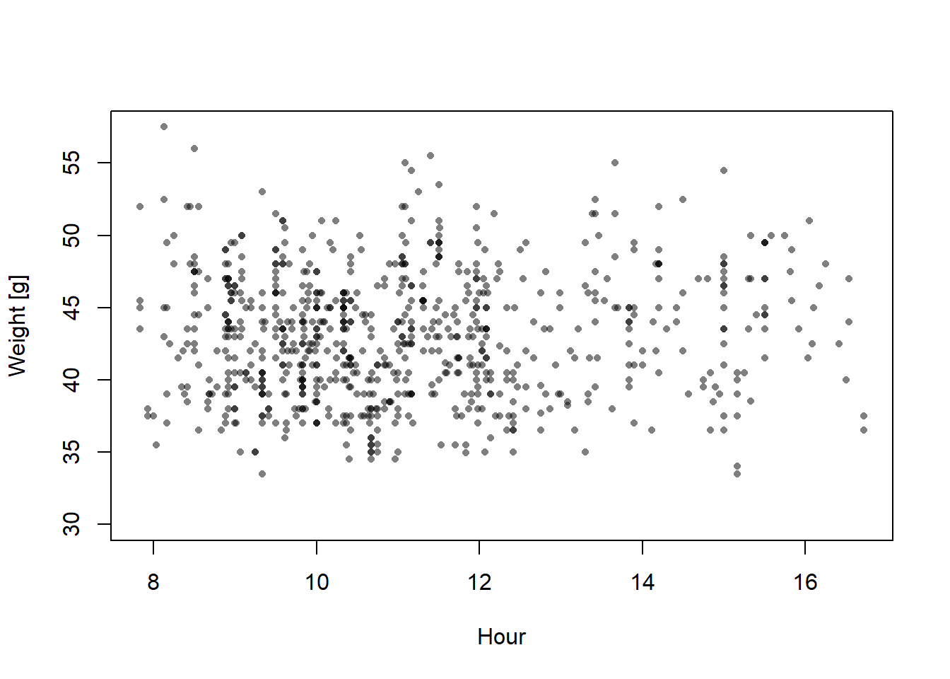

13.2.4 Fit the regression using lm

Theory

mod <- lm(weight~time.num, data=dat)
mod

## 
## Call:
## lm(formula = weight ~ time.num, data = dat)
## 
## Coefficients:
## (Intercept)     time.num  
##     41.6403       0.1263

plot(dat$time.num, dat$weight, xlab="Hour", ylab="Weight [g]", pch=16, col=rgb(0,0,0,0.5), cex=0.7)
abline(mod, col="brown")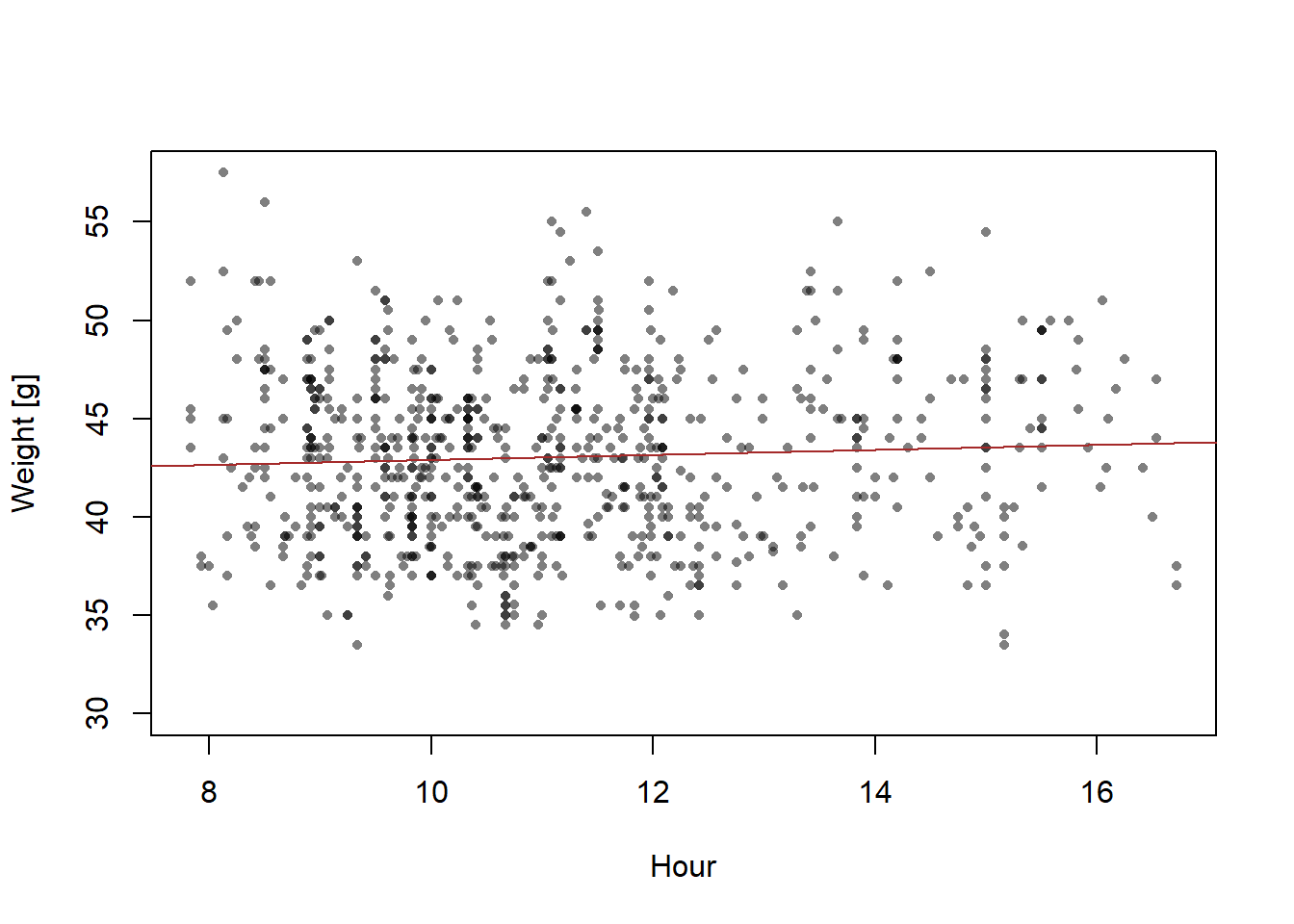

• What does the function lm do?

• What are the model parameters and what are their estimates?

• How does the formula of the regression line look like?

13.2.5 Check the model assumptions

Theory

par(mfrow=c(2,2))
plot(mod)

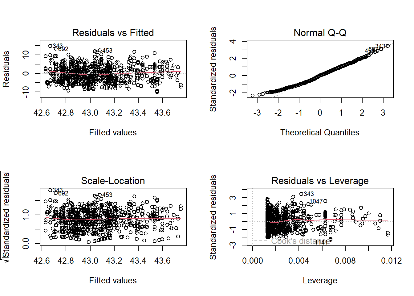
Figure 13.1: Diagnostic residual plots of a normal linear model fitted to simulated data, thus model assumptions are perfectly met. See text for explanation.

• Would you trust this model? Do you think the model assumptions are met?

• Which structures of the data could violate the model assumptions?

13.2.6 Drawing Conclusions

To answer the question about how strongly \(y\) is related to \(x\) taking into account statistical uncertainty we look at the estimated slope \(\beta_{1}\) and its standard error (SE). The slope \(\beta_{1}\) measures how much \(y\) increases in average when \(x\) is increased by 1 unit. The value of \(\beta_{1}\) is calculated from the data at hand. It is therefore, a characteristics of the specific data. However, we would like to draw our conclusions more generally, i.e. also in future, for new data, we expect that \(y\) increases by \(\beta_{1}\) if \(x\) increases by 1. However for these unmeasured, future data \(\beta_{1}\) may look differently. No statistical method can exactly predict how \(\beta_{1}\) will look for future data. However, if we assume that the model assumptions reflect the real world reasonable well, we can use the standard error (SE) as an estimate of how far away in average the estimated \(\beta_{1}\) may be from the underlying true value, i.e. a \(\beta_{1}\) that we would measure if we had sampled a very high number of (i.e., all) observations.

summary(mod)

## 
## Call:
## lm(formula = weight ~ time.num, data = dat)
## 
## Residuals:
##      Min       1Q   Median       3Q      Max 
## -10.0561  -3.3193  -0.0361   3.0881  14.8323 
## 
## Coefficients:
##             Estimate Std. Error t value Pr(>|t|)    
## (Intercept) 41.64032    0.88299  47.159   <2e-16 ***
## time.num     0.12631    0.07829   1.613    0.107    
## ---
## Signif. codes:  0 '***' 0.001 '**' 0.01 '*' 0.05 '.' 0.1 ' ' 1
## 
## Residual standard error: 4.31 on 779 degrees of freedom
##   (279 Beobachtungen als fehlend gelöscht)
## Multiple R-squared:  0.003331,   Adjusted R-squared:  0.002051 
## F-statistic: 2.603 on 1 and 779 DF,  p-value: 0.1071

• What does the output of the function summary tell us?

To draw a 95% compatibility interval around the regression line, we first define new x-values for which we would like to have the fitted values (about 100 points across the range of x will produce smooth-looking lines when connected by line segments). We save these new x-values within the new data.frame newdat. (Fig. 13.2).

# Calculate 95% CI
range(dat$time.num, na.rm=TRUE)

## [1]  7.833333 16.716667

newdat <- data.frame(time.num = seq(7, 17, length=100))
newdat$fit <- predict(mod, newdata=newdat)
newdat$lwr <- predict(mod, interval="confidence", newdata=newdat)[,2]
newdat$upr <- predict(mod, interval="confidence", newdata=newdat)[,3]


plot(dat$time.num, dat$weight, xlab="Hour", ylab="Weight [g]", pch=16, col=rgb(0,0,0,0.5), cex=0.7)
lines(newdat$time.num, newdat$fit, lwd=2, col="brown")
lines(newdat$time.num, newdat$lwr, lwd=2, lty=3, col="brown")
lines(newdat$time.num, newdat$upr, lwd=2, lty=3, col="brown")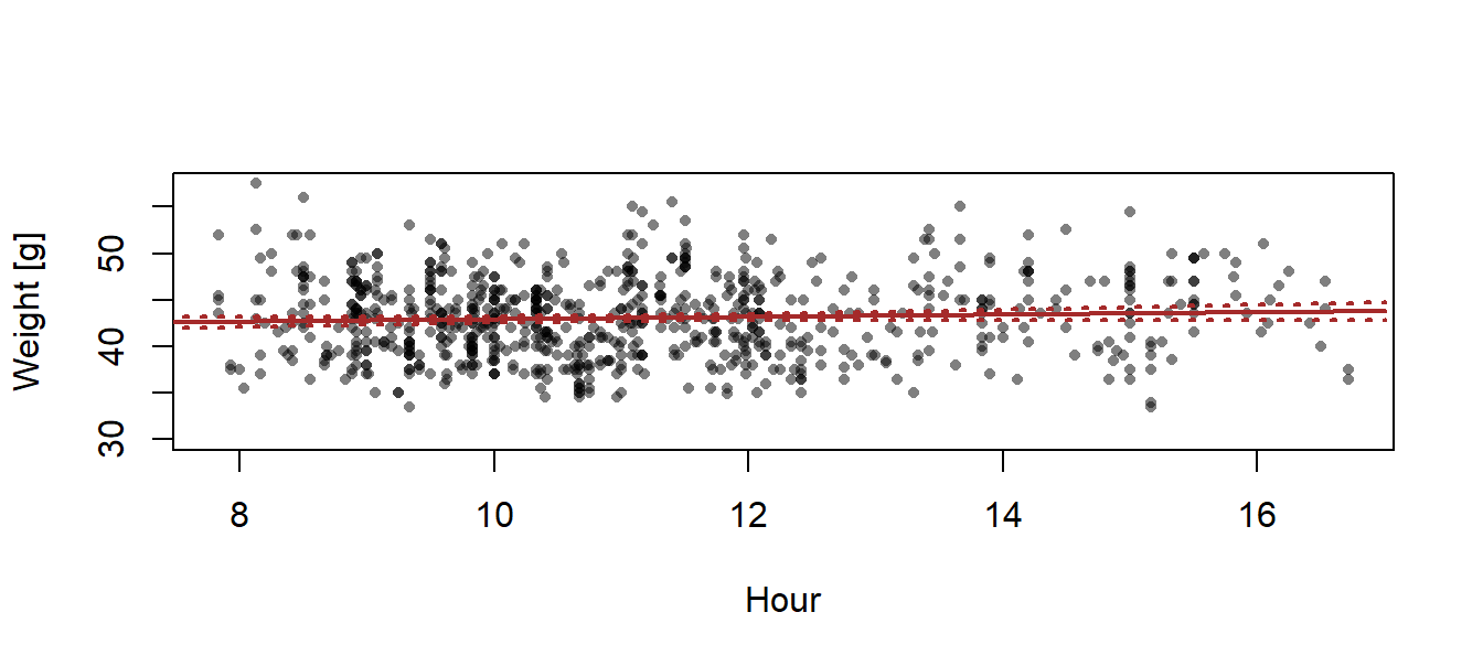

Figure 13.2: Regression with 95% credible interval of the posterior distribution of the fitted values.

# Make the same plot using ggplot
#regplot <- 
#  ggplot(dat, aes(x = x, y = y)) +
#  geom_point() +
#  geom_abline(intercept = coef(mod)[1], slope=coef(mod)[2], lwd=1, col="blue") +
#  geom_line(data = newdat, aes(x = x, y = CrI_lo), lty = 3) +
#  geom_line(data = newdat, aes(x = x, y = CrI_up), lty = 3) +
#  labs(x = "Predictor (x)", y = "Outcome (y)")
#regplot

The uncertainty interval measures statistical uncertainty of the regression line, but it does not describe how new observations would scatter around the regression line. If we want to describe where future observations will be, we have to report the prediction interval (see online book, posterior predictive distribution), or present the data within the plot of the regression line.

• How would you describe the results for a paper?